Inhoud
Newtons methode
De waarheid is veel te ingewikkeld om iets anders dan benaderingen toe te laten.
– John Von Neumann
Oplossing vinden met meetkunde
De methode van Newton om vergelijkingen op te lossen is een andere numerieke methode om een vergelijking $f(x) = 0$ op te lossen. Zij is gebaseerd op de meetkunde van een kromme, met behulp van de raaklijnen aan een kromme. Als zodanig vereist zij calculus, met name differentiatie.
Ruwweg komt het idee van de methode van Newton op het volgende neer. We zoeken een oplossing voor $f(x) = 0$. Dat wil zeggen, we willen het rode gestippelde punt in het plaatje hieronder vinden.
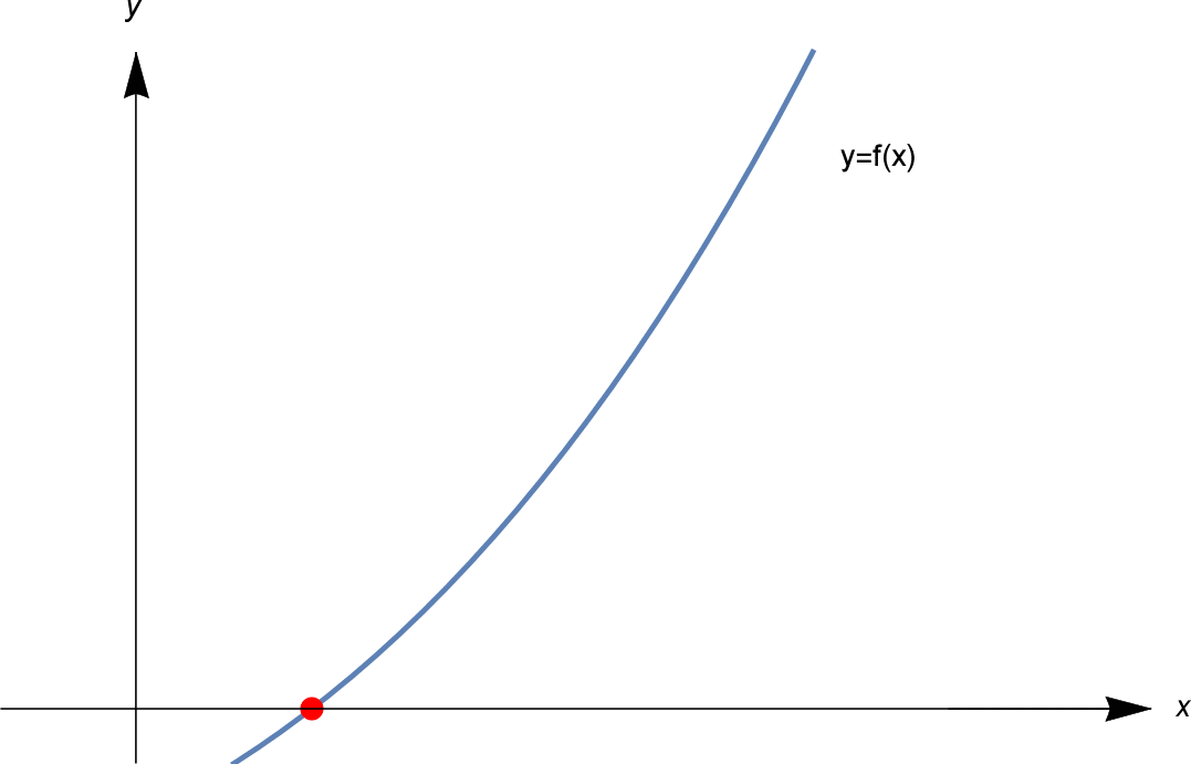
We beginnen met een eerste schatting $x_1$. We berekenen $f(x_1)$. Als $f(x_1) = 0$, hebben we veel geluk, en hebben we een oplossing. Maar hoogstwaarschijnlijk is $f(x_1)$ niet nul. Laat $f(x_1) = y_1$, zoals getoond.
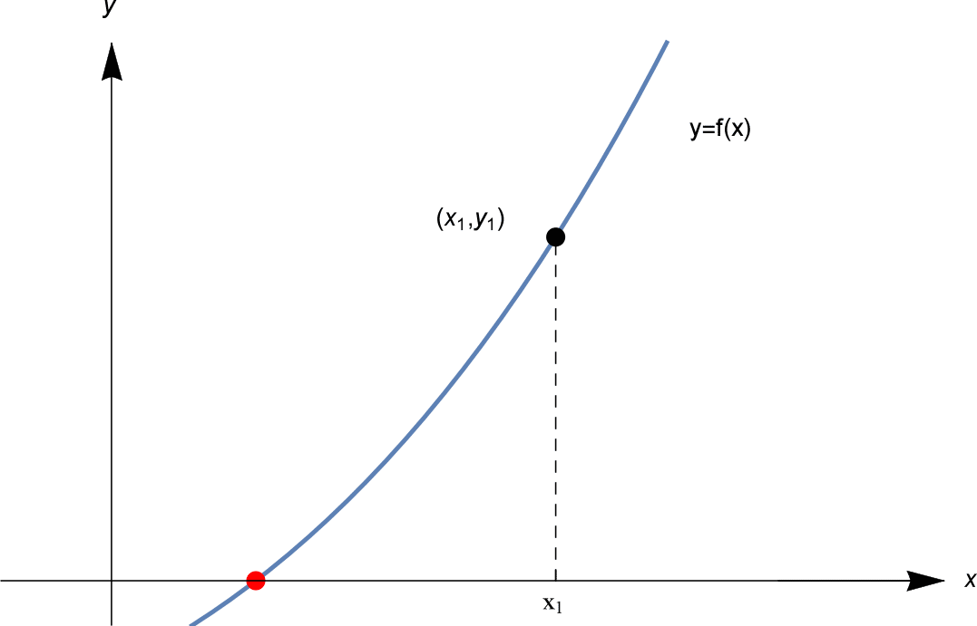
We gaan nu op zoek naar een betere schatting. Hoe vinden we die betere gok? De truc van de methode van Newton is om een raaklijn aan de grafiek $y=f(x)$ te tekenen in het punt $(x_1, y_1)$. Zie hieronder.
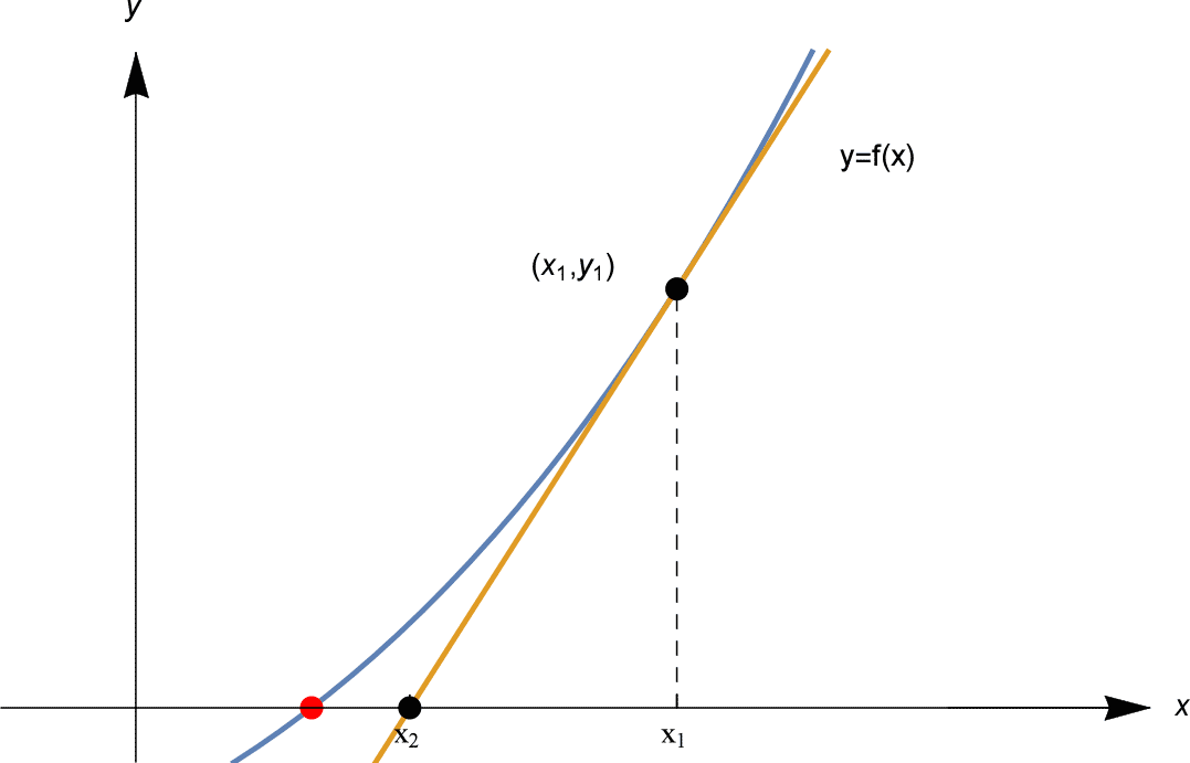
Deze raaklijn is een goede lineaire benadering van $f(x)$ in de buurt van $x_1$, dus onze volgende gok $x_2$ is het punt waar de raaklijn de $x$-as snijdt, zoals hierboven te zien is.
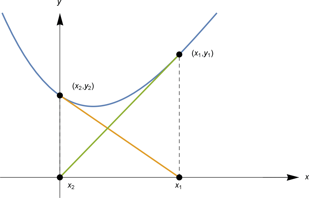
Dan gaan we volgens dezelfde methode te werk. We berekenen $y_2 = f(x_2)$; als deze nul is, zijn we klaar. Zo niet, dan tekenen we de raaklijn aan $y=f(x)$ bij $(x_2, y_2)$, en onze volgende gok $x_3$ is het punt waar deze raaklijn de $x$-as snijdt. Zie hieronder.
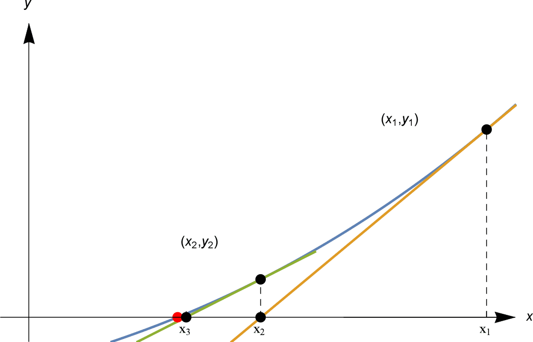
In de figuur hiernaast naderen $x_1, x_2, x_3$ snel het rode oplossingspunt!
Door op deze manier verder te gaan, vinden we punten $x_1, x_2, x_3, x_4, \ldots$ die een oplossing benaderen. Deze methode om een oplossing te vinden is de methode van Newton.
Zoals we zullen zien, kan de methode van Newton een zeer efficiënte methode zijn om een oplossing van een vergelijking te benaderen – als het werkt.
De belangrijkste berekening
Zoals onze inleiding hierboven liet zien, is de belangrijkste berekening in elke stap van de methode van Newton te vinden waar de raaklijn aan $y=f(x)$ in het punt $(x_1, y_1)$ de $x$-as snijdt.
Laten we dit $x$-afsnijpunt eens vinden. De raaklijn die we zoeken gaat door het punt $(x_1, y_1)$ en heeft als gradiënt $f'(x_1)$.
Ontdek dat, gegeven de gradiënt $m$ van een lijn, en een punt $(x_0, y_0)$ erop, de lijn vergelijking heeft
In onze situatie heeft de lijn gradiënt $f'(x_1)$, en gaat door $(x_1, y_1)$, dus heeft vergelijking
Zie het diagram hieronder.
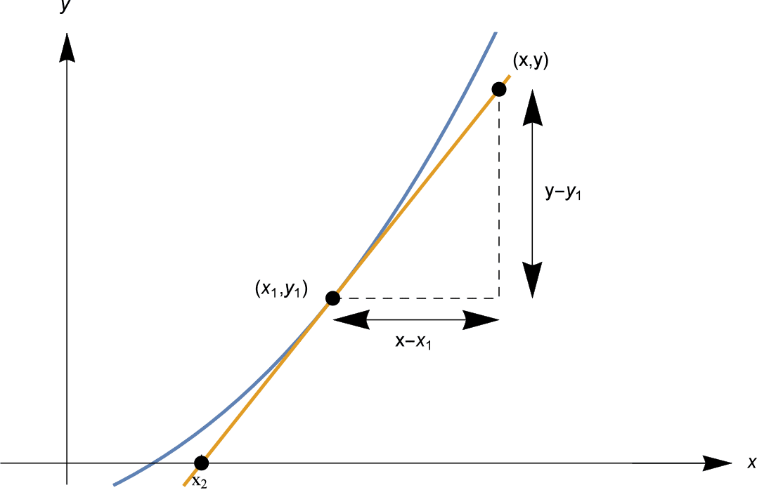
Zetten we $y=0$, dan vinden we het $x$-afsnijpunt als
Het algoritme
We kunnen de methode van Newton nu algebraïsch beschrijven. Uitgaande van $x_1$ toont bovenstaande berekening aan dat als we de raaklijn aan de grafiek $y=f(x)$ construeren bij $x=x_1$, deze raaklijn een $x$-afsnijpunt heeft dat gegeven wordt door
Dan, uitgaande van $x_2$ voeren we dezelfde berekening uit, en bekomen we de volgende benadering $x_3$ als
Dezelfde berekening geldt in elke fase: dus vanaf de $n
Newtons methode
Laat $f: \mathbb{R} \rrechtsarrow \mathbb{R}$ een differentieerbare functie zijn. We zoeken een oplossing van $f(x) = 0$, uitgaande van een beginschatting $x = x_1$.
Bij de $n Het is echter belangrijk op te merken dat de methode van Newton niet altijd werkt. Er kunnen verschillende dingen fout gaan, zoals we zo dadelijk zullen zien.
De methode van Newton gebruiken
Net als bij de bisectiemethode benaderen we enkele bekende constanten.
Voorbeeld
Gebruik de methode van Newton om bij benadering een oplossing te vinden voor $x^2 – 2 = 0$, uitgaande van een beginschatting $x_1 =2$. Na 4 iteraties, hoe dicht ligt de benadering bij $x_1 =2$?
Oplossing
Laat $f(x) = x^2 – 2$, dus $f'(x) = 2x$. Bij stap 1 hebben we $x_1 = 2$ en we berekenen $f(x_1) = 2^2 – 2 = 2$ en $f'(x_1) = 4$, dus
Bij stap 2, uit $x_2 = \frac{3}{2}$ berekenen we $f(x_2) = \frac{1}{4}$ en $f'(x_2) = 3$, dus
Bij stap 3, uit $x_3 = \frac{17}{12}$ hebben we $f(x_3) = \frac{1}{144}$ en $f'(x_3) = \frac{17}{6}$, dus
Bij stap 4, berekenen we uit $x_4 = \frac{577}{408}$ $f(x_4) = \frac{1}{166,464}$ en $f'(x_4) = \frac{577}{204}$, dus
In feite is tot 12 decimalen $\sqrt{2} \1,414213562373$. Dus na 4 iteraties is de benaderde oplossing $x_5$ tot 11 decimalen gelijk aan $\sqrt{2}$. Het verschil tussen $x_5$ en $\sqrt{2}$ is
De methode van Newton in het bovenstaande voorbeeld is veel sneller dan het bisectie-algoritme! In slechts 4 iteraties hebben we 11 decimalen nauwkeurigheid! De volgende tabel laat zien hoeveel decimalen nauwkeurigheid we hebben in elke $x_n$.
| $n$ | $1$ | $2$ | $3$ | $4$ | $5$ | $6$ | $7$ |
| # decimale plaatsen nauwkeurigheid in | $0$ | $0$ | $2$ | $5$ | $11$ | $23$ | $47$ |
Het aantal decimale plaatsen van nauwkeurigheid verdubbelt ongeveer bij elke iteratie!
Oefening 10
(Moeilijker.) Dit probleem onderzoekt deze verdubbeling van nauwkeurigheid:
- Bereken eerst dat $x_{n+1} = \frac{x_n}{2} + \frac{1}{x_n}$ en dat, als $y_n = x_n – \sqrt{2}$, dan $y_{n+1} = \frac{y_n^2}{2(\sqrt{2} + y_n)}$.
- Ontdek dat, als $x_1 > 0$ (resp. $x_1 \sqrt{2}$ (resp. $x_n
- Laat zien dat als $0
- Laat zien dat, voor $n \geq 2$, als $x_n$ verschilt van $\sqrt{2}$ met minder dan $10^{-k}$, dan $x_{n+1}$ verschilt van $\sqrt{2}$ met minder dan $10^{-2k}$.
Voorbeeld
Vind een benadering van $\pi$ door met de methode van Newton $\sin x = 0$ voor 3 iteraties op te lossen, uitgaande van $x_1=3$. Tot op hoeveel decimalen nauwkeurig is de benaderde oplossing?
Oplossing
Laat $f(x) = \sin x$, dus $f'(x) = \cos x$. We berekenen $x_2, x_3, x_4$ direct met de formule
We berekenen elke $x_n$ direct tot 25 decimalen, voor 3 iteraties:
Tot 25 decimalen, $³pi = 3.1415926535897932384626433$; $x_4$ komt overeen met 24 plaatsen.
In het bovenstaande voorbeeld is de convergentie nog sneller dan in ons $\sqrt{2}$ voorbeeld. Het aantal decimalen nauwkeurigheid verdrievoudigt ruwweg bij elke iteratie!
| $n$ | $1$ | $2$ | $3$ | $4$ | $5$ |
| # decimale plaatsen nauwkeurigheid in $x_n$ | $0$ | $2$ | $9$ | $24$ | $87$ |
Oefening 11
Vind alle oplossingen van de vergelijking $x_n$ tot 9 decimalen met behulp van de methode van Newton. Vergelijk de convergentie met die van de bisectiemethode in opgave 5.
Wat kan er misgaan
Hoewel de methode van Newton fantastisch goede benaderingen van een oplossing kan geven, kunnen er verschillende dingen misgaan. We bekijken nu enkele van deze minder gelukkige gedragingen.
Het eerste probleem is dat de $x_n$ misschien niet eens gedefinieerd is!
Voorbeeld
Vind een benaderende oplossing voor $x_1 = \frac{\pi}{2}$ met behulp van de methode van Newton, uitgaande van $x_1 = \frac{\pi}{2}$.
Oplossing
We stellen $f(x) = \sin x$, dus $f'(x) = \cos x$. Nu is $x_2 = x_1 – \frac{f(x_1)}{f'(x_1)}$, maar $f'(x_1) = \cos \frac{\pi}{2} = 0$, dus is $x_2$ niet gedefinieerd, en dus ook geen van de volgende $x_n$.
Dit probleem doet zich steeds voor als $f'(x_n) = 0$. Als $x_n$ een stationair punt van $f$ is, probeert Newtons methode door nul te delen – en mislukt.
Het volgende voorbeeld illustreert dat zelfs als de “benaderde oplossingen” $x_n$ bestaan, zij een oplossing misschien niet erg goed “benaderen”.
Voorbeeld
Benader een oplossing voor $-x^3 + 4x^2 – 2x + 2 = 0$ met behulp van de methode van Newton vanaf $x_1 = 0$.
Oplossing
Laat $f(x) = -x^3 + 4x^2 – 2x + 2$, dus $f'(x) = -3x^2 + 8x – 2$. Uitgaande van $x_1 = 0$, hebben we
We hebben nu gevonden dat $x_3 = x_1 = 0$. De berekening voor $x_4$ is dan precies dezelfde als voor $x_2$, dus $x_4 = x_2 = 1$. Dus $x_n = 0$ voor alle oneven $n$, en $x_n = 1$ voor alle even $n$. De $x_n$ zitten opgesloten in een cyclus, waarbij ze afwisselen tussen twee waarden.
In bovenstaand voorbeeld is er eigenlijk een oplossing, $x = \frac{1}{3} \links( 4 + \sqrt{10} + \sqrt{100} rechts) \sim 3.59867$. Onze “benaderende oplossingen” $x_n$ benaderen het niet, in plaats daarvan fietsen ze zoals hieronder geïllustreerd.
Het derde probleem laat zien dat alle $x_n$ steeds verder van een oplossing af kunnen komen te liggen!
Voorbeeld
Vind bij benadering een oplossing voor $x_1 = 3$, met behulp van de methode van Newton.
Oplossing
Laat $f(x) = \arctan x$, dus $f'(x) = \frac{1}{1+x^2}$. Uit $x_1 = 3$ kunnen we achtereenvolgens $x_2, x_3, \ldots$ berekenen. We schrijven ze in 2 decimalen.
begin{align*}x_2 &= x_1 – \frac{f(x_1)}{f'(x_1)} = 3 – \frac{arctan 3}{\frac{1}{1+3^2}} = 3 – 10 \arctan 3 \sim -9,49. \x_3 &= x_2 – \frac{f(x_2)}{f'(x_2)} \x_4 &= x_3 – \frac{f(x_3)}{f'(x_3)} \sim -23,905.94
De “benaderingen” $x_n$ divergeren snel naar oneindig.
Het bovenstaande voorbeeld lijkt misschien een beetje dwaas, omdat het vinden van een exacte oplossing voor $x=0$ niet moeilijk is: de oplossing is $x=0$! Maar soortgelijke problemen zullen zich voordoen bij toepassing van de methode van Newton op elke kromme met een vergelijkbare vorm. Het feit dat $f'(x_n)$ dicht bij nul ligt, betekent dat de raaklijn dicht bij horizontaal ligt, en dus ver weg kan lopen om bij het $x$ -uiteinde van $x_{n+1}$ uit te komen.
Sensitieve afhankelijkheid van beginvoorwaarden
Soms kan de keuze van de beginvoorwaarden heel klein zijn, maar toch tot een radicaal andere uitkomst leiden in Newtons methode.
Overweeg het oplossen van $f(x) = 2x – 3x^2 + x^3 = 0$. Het is mogelijk om de kubus te ontbinden in factoren, $f(x) = x(x-1)(x-2)$, zodat de oplossingen gewoon $x=0, 1$ en $2$ zijn.
Als we de methode van Newton toepassen met verschillende beginschattingen $x_1$, komen we misschien uit bij een van deze drie oplossingen….of ergens anders.
Zoals hierboven geïllustreerd, passen we de methode van Newton toe uitgaande van $x_1 = 1.4$ en $x_1 = 1.5$. Uitgaande van $x_1 = 1.4 = \frac{7}{5}$ berekenen we, tot 6 decimalen achter de komma,
en de $x_n$ convergeren naar de oplossing $x=1$. En uitgaande van $x_1 = 1.5$ berekenen we $x_2 = 0$, een exacte oplossing, dus alle $x_3 = x_4 = \cdots = 0$.
We kunnen ons dan afvragen: waar, tussen de beginschattingen $x_1 = 1.4$ en $x_1 = 1.5$, schakelt de reeks over van het benaderen van $x=1$, naar het benaderen van $x=0$?
We vinden dat de beginschatting $x_1 = 1.45$ zich op dezelfde manier gedraagt als $1.5$: de reeks $x_n$ nadert de oplossing $x = 0$. Anderzijds gedraagt de beginschatting $x_1 = 1.44$ zich als $1.4$: $x_n$ nadert de oplossing $x=1$. De uitkomst lijkt te schakelen ergens tussen de beginschattingen $x_1 = 1.44$ en $x_1 = 1.45$. Met wat meer berekeningen kunnen we verder gaan en vinden we dat de omschakeling ergens tussen $x_1 = 1.447$ en $x_1 = 1.448$ gebeurt. De berekeningen (tot 3 decimalen) vanaf deze beginwaarden staan in de tabel hieronder.
Dus, als we $x_1 = 1.4475$ proberen, convergeert de $x_n$ dan naar de oplossing $x=1$ of $x=0$? Het antwoord is geen van beide: zoals uit de tabel blijkt, convergeert hij naar de oplossing $x=2$!
| $x_1$ | $1.4$ | $1,44$ | $1,447$ | $1,4475$ | $1,448$ | $1,45$ | $1,447$ | $1,4475$ | $1,448$ | $1.5$ | $x_2$ | $0,754$ | $0,594$ | $0,554$ | $0,551$ | $0.548$ | $0,536$ | $0$ |
| $x_3$ | $1,036$ | $1,266$ | $1,440$ | $1.458$ | $1.477$ | $1.567$ | $0$ | |||
| $x_4$ | $1.000$ | $0.952$ | $0.596$ | $0.484$ | $0.317$ | $-9.156$ | $0$ | |||
| $x_5$ | $1.000$ | $1.000$ | $1.260$ | $2.370$ | $-0.598$ | $-5.793$ | $0$ | |||
| $x_6$ | $1.000$ | $1.000$ | $0.956$ | $2.111$ | $-0.225$ | $-3.562$ | $0$ | |||
| $x_7$ | $1.000$ | $1.000$ | $1.000$ | $2.111$ | $-0.225$ | $-3.562$ | $0$ | |||
| $x_8$ | $1.000$ | $1.000$ | $1.000$ | $2.000$ | $-0.003$ | $-1.135$ | $0$ | |||
| $x_9$ | $1.000$ | $1.000$ | $1.000$ | $1.000$ | $1.000$ | $1.000$ | $2.000$ | $0.000$ | $-0.536$ | $0$ |
| $x_{10}$ | $1.000$ | $1.000$ | $1.000$ | $2.000$ | $0.000$ | $-0.192$ | $0$ | |||
| $x_{11}$ | $1.000$ | $1.000$ | $1.000$ | $2.000$ | $0.000$ | $-0.038$ | $0$ | |||
| $x_{12}$ | $1.000$ | $1.000$ | $1.000$ | $2.000$ | $0.000$ | $-0.002$ | $0$ |
Verder, als we $x_1 = 1 + \frac{1}{\sqrt{5}} \sim 1,447214$, vinden we weer ander gedrag! Wat blijkt,
dus $x_1 = x_3$ en de $x_n$ wisselen tussen deze twee waarden.
Oefening 12
Verklaar dat als $f(x) = 2x – 3x^2 + x^3 = x(x-1)(x-2)$ en $x_1 = 1 + \frac{1}{\sqrt{5}}$, dan is $x_2 = 1 – \frac{1}{\sqrt{5}}$ en $x_3 = 1 + \frac{1}{\sqrt{5}} = x_1$.
Er is dus geen eenvoudige overgang van die waarden van $x_1$ die leiden tot de oplossing $x = 1$ en $x=0$. Het gedrag van de Newton-methode hangt uiterst gevoelig af van de beginwaarde $x_1$. We hebben immers slechts een handvol waarden voor $x_1$ uitgeprobeerd, en hebben slechts het topje van de ijsberg van dit gedrag gezien.
In de paragraaf Links vooruit onderzoeken we dit gedrag verder, en laten we enkele plaatjes zien van deze gevoelige afhankelijkheid van de beginvoorwaarden, die duidt op wiskundige chaos. Afbeeldingen die het gedrag van de methode van Newton illustreren tonen het ingewikkelde detail van een fractal.
De methode van Newton aan het werk zetten
In het algemeen is het moeilijk om precies aan te geven wanneer de methode van Newton goede benaderingen zal opleveren van een oplossing van $f(x) = 0$. Maar we kunnen de volgende opmerkingen maken, die een samenvatting zijn van onze eerdere waarnemingen.
- Als $f'(x_n) = 0$ dan faalt de methode van Newton onmiddellijk, omdat hij probeert te delen door nul.
- De “benaderingen” $x_1, x_2, x_3, \ldots$ kunnen ronddraaien, in plaats van naar een oplossing te convergeren.
- De “benaderingsoplossingen” $x_1, x_2, x_3, \ldots$ kunnen zelfs naar oneindig divergeren. Dit probleem doet zich voor als $f'(x_n)$ klein is, maar niet nul.
- Het gedrag van Newtons methode kan extreem gevoelig afhangen van de keuze van $x_1$, en leiden tot een chaotische dynamiek.
Een handige vuistregel is echter de volgende:
- Voorstel dat je een grafiek kunt schetsen van $y=f(x)$, en dat je bij benadering de plaats van een oplossing kunt zien, en dat $f'(x)$ niet te klein is in de buurt van die oplossing. Als je dan $x_1$ in de buurt van die oplossing neemt, en weg van andere oplossingen of kritieke punten, zal de methode van Newton $x_n$ opleveren die snel naar de oplossing convergeren.
Volgende pagina – Links vooruit – Snelheid van het bisectiealgoritme
|
|
Deze materialen zijn ontwikkeld in samenwerking met de Victorian Curriculum and Assessment Authority. © VCAA en The University of Melbourne namens AMSI 2015 |
Bijdragers Gebruiksvoorwaarden |
th benadering $x_n$, wordt de volgende benadering gegeven door\
Formeel ziet het algoritme van Newton er als volgt uit.
Newton’s method
Let $f: \mathbb{R} \rightarrow \mathbb{R}$ be a differentiable function. We seek a solution of $f(x) = 0$, starting from an initial estimate $x = x_1$.
At the $n$’th step, given $x_n$, compute the next approximation $x_{n+1}$ by
\
Some comments about this algorithm:
- Often, Newton’s method works extremely well, and the $x_n$ converge rapidly to a solution. However, it’s important to note that Newton’s method does not always work. Several things can go wrong, as we will see shortly.
- Note that if $f(x_n) = 0$, so that $x_n$ is an exact solution of $f(x) = 0$, then the algorithm gives $x_{n+1} = x_n$, and in fact all of $x_n, x_{n+1}, x_{n+2}, x_{n+3}, \ldots$ will be equal. If you have an exact solution, Newton’s method will stay on that solution!
- While the bisection method only requires $f$ to be continuous, Newton’s method requires the function $f$ to be differentiable. This is necessary for $f$ to have a tangent line.
Using Newton’s method
As we did with the bisection method, let’s approximate some well-known constants.
Example
Use Newton’s method to find an approximate solution to $x^2 – 2 = 0$, starting from an initial estimate $x_1 =2$. After 4 iterations, how close is the approximation to $\sqrt{2}$?
Solution
Let $f(x) = x^2 – 2$, so $f'(x) = 2x$. At step 1, we have $x_1 = 2$ and we calculate $f(x_1) = 2^2 – 2 = 2$ and $f'(x_1) = 4$, so
\
At step 2, from $x_2 = \frac{3}{2}$ we calculate $f(x_2) = \frac{1}{4}$ and $f'(x_2) = 3$, so
\
At step 3, from $x_3 = \frac{17}{12}$ we have $f(x_3) = \frac{1}{144}$ and $f'(x_3) = \frac{17}{6}$, so
\
At step 4, from $x_4 = \frac{577}{408}$ we calculate $f(x_4) = \frac{1}{166,464}$ and $f'(x_4) = \frac{577}{204}$, so
\
In fact, to 12 decimal places $\sqrt{2} \sim 1.414213562373$. So after 4 iterations, the approximate solution $x_5$ agrees with $\sqrt{2}$ to 11 decimal places. The difference between $x_5$ and $\sqrt{2}$ is
\
Newton’s method in the above example is much faster than the bisection algorithm! In only 4 iterations we have 11 decimal places of accuracy! The following table illustrates how many decimal places of accuracy we have in each $x_n$.
| $n$ | $1$ | $2$ | $3$ | $4$ | $5$ | $6$ | $7$ |
| # decimal places accuracy in | $0$ | $0$ | $2$ | $5$ | $11$ | $23$ | $47$ |
The number of decimal places of accuracy approximately doubles with each iteration!
Exercise 10
(Harder.) This problem investigates this doubling of accuracy:
- First calculate that $x_{n+1} = \frac{x_n}{2} + \frac{1}{x_n}$ and that, if $y_n = x_n – \sqrt{2}$, then $y_{n+1} = \frac{y_n^2}{2(\sqrt{2} + y_n)}$.
- Show that, if $x_1 > 0$ (resp. $x_1 \sqrt{2}$ (resp. $x_n
- Show that if $0
- Show that, for $n \geq 2$, if $x_n$ differs from $\sqrt{2}$ by less than $10^{-k}$, then $x_{n+1}$ differs from $\sqrt{2}$ by less than $10^{-2k}$.
Example
Find an approximation to $\pi$ by using Newton’s method to solve $\sin x = 0$ for 3 iterations, starting from $x_1=3$. To how many decimal places is the approximate solution accurate?
Solution
Let $f(x) = \sin x$, so $f'(x) = \cos x$. We compute $x_2, x_3, x_4$ directly using the formula
\
We compute directly each $x_n$ to 25 decimal places, for 3 iterations:
\
To 25 decimal places, $\pi = 3.1415926535897932384626433$; $x_4$ agrees to 24 places.
In the above example, convergence is even more rapid than for our $\sqrt{2}$ example. The number of decimal places accuracy roughly triples with each iteration!
| $n$ | $1$ | $2$ | $3$ | $4$ | $5$ |
| # decimal places accuracy in $x_n$ | $0$ | $2$ | $9$ | $24$ | $87$ |
Exercise 11
Find all solutions to the equation $\cos x = x$ to 9 decimal places using Newton’s method. Compare the convergence to what you obtained with the bisection method in exercise 5.
What can go wrong
While Newton’s method can give fantastically good approximations to a solution, several things can go wrong. We now examine some of this less fortunate behaviour.
The first problem is that the $x_n$ may not even be defined!
Example
Find an approximate solution to $\sin x = 0$ using Newton’s method starting from $x_1 = \frac{\pi}{2}$.
Solution
We set $f(x) = \sin x$, so $f'(x) = \cos x$. Now $x_2 = x_1 – \frac{f(x_1)}{f'(x_1)}$, but $f'(x_1) = \cos \frac{\pi}{2} = 0$, so $x_2$ is not defined, hence nor are any subsequent $x_n$.
This problem occurs whenever when $f'(x_n) = 0$. If $x_n$ is a stationary point of $f$, then Newton’s method attempts to divide by zero — and fails.
The next example illustrates that even when the “approximate solutions” $x_n$ exist, they may not “approximate” a solution very well.
Example
Approximate a solution to $-x^3 + 4x^2 – 2x + 2 = 0$ using Newton’s method from $x_1 = 0$.
Solution
Let $f(x) = -x^3 + 4x^2 – 2x + 2$, so $f'(x) = -3x^2 + 8x – 2$. Starting from $x_1 = 0$, we have
\
We have now found that $x_3 = x_1 = 0$. The computation for $x_4$ is then exactly the same as for $x_2$, so $x_4 = x_2 = 1$. Thus $x_n = 0$ for all odd $n$, and $x_n = 1$ for all even $n$. The $x_n$ are locked into a cycle, alternating between two values.
In the above example, there is actually a solution, $x = \frac{1}{3} \left( 4 + \sqrt{10} + \sqrt{100} \right) \sim 3.59867$. Our “approximate solutions” $x_n$ fail to approximate it, instead cycling as illustrated below.
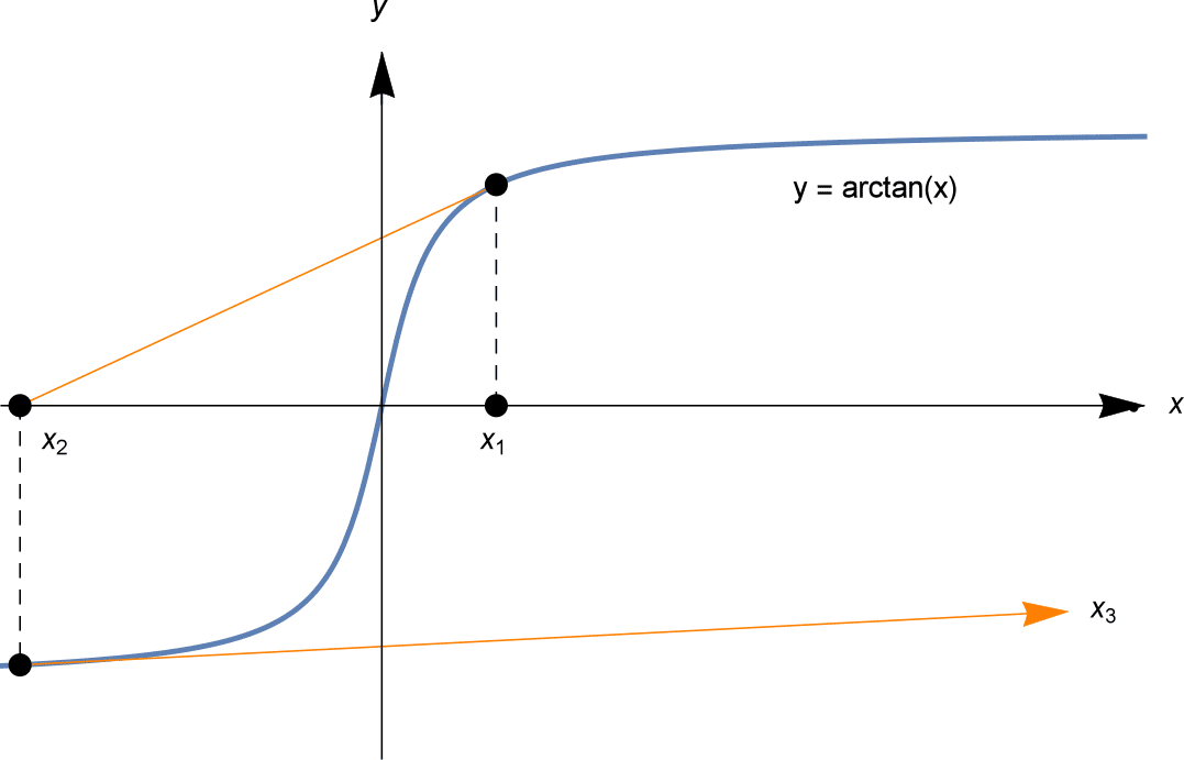
The third problem shows that all $x_n$ can get further and further away from a solution!
Example
Find an approximate solution to $\arctan x = 0$, using Newton’s method starting at $x_1 = 3$.
Solution
Let $f(x) = \arctan x$, so $f'(x) = \frac{1}{1+x^2}$. From $x_1 = 3$ we can compute successively $x_2, x_3, \ldots$. We write them to 2 decimal places.
\begin{align*}x_2 &= x_1 – \frac{f(x_1)}{f'(x_1)} = 3 – \frac{\arctan 3}{\frac{1}{1+3^2}} = 3 – 10 \arctan 3 \sim -9.49. \\x_3 &= x_2 – \frac{f(x_2)}{f'(x_2)} \sim 124.00 \\x_4 &= x_3 – \frac{f(x_3)}{f'(x_3)} \sim -23,905.94\end{align*}
The “approximations” $x_n$ rapidly diverge to infinity.
The above example may seem a little silly, since finding an exact solution to $\arctan x = 0$ is not difficult: the solution is $x=0$! But similar problems will happen applying Newton’s method to any curve with a similar shape. The fact that $f'(x_n)$ is close to zero means the tangent line is close to horizontal, and so may travel far away to arrive at its $x$-intercept of $x_{n+1}$.
Sensitive dependence on initial conditions
Sometimes the choice of initial conditions can be ever so slight, yet lead to a radically different outcome in Newton’s method.
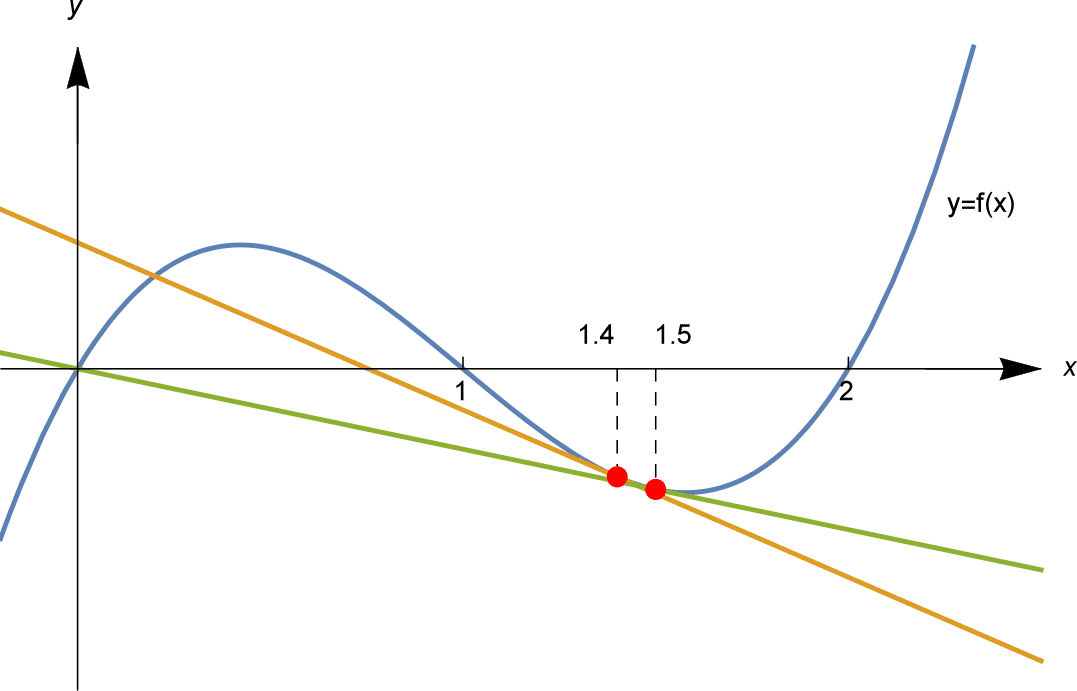
Consider solving $f(x) = 2x – 3x^2 + x^3 = 0$. It’s possible to factorise the cubic, $f(x) = x(x-1)(x-2)$, so the solutions are just $x=0, 1$ and $2$.
If we apply Newton’s method with different starting estimates $x_1$, we might end up at any of these three solutions… or somewhere else.
As illustrated above, we apply Newton’s method starting from $x_1 = 1.4$ and $x_1 = 1.5$. Starting from $x_1 = 1.4 = \frac{7}{5}$ we compute, to 6 decimal places,
\
and the $x_n$ converge to the solution $x=1$. And starting from $x_1 = 1.5$ we compute $x_2 = 0$, an exact solution, so all $x_3 = x_4 = \cdots = 0$.
We might then ask: where, between the initial estimates $x_1 = 1.4$ and $x_1 = 1.5$, does the sequence switch from approaching $x=1$, to approaching $x=0$?
We find that the the initial estimate $x_1 = 1.45$ behaves similarly to $1.5$: the sequence $x_n$ approaches the solution $x = 0$. On the other hand, taking $x_1 = 1.44$ behaves similarly to $1.4$: $x_n$ approaches the solution $x=1$. The outcome seems to switch somewhere between the initial estimates $x_1 = 1.44$ and $x_1 = 1.45$. With some more computations, we can narrow down further and find that the switch happens somewhere between $x_1 = 1.447$ and $x_1 = 1.448$. The computations (to 3 decimal places) from these initial values are shown in the table below.
So, if we try $x_1 = 1.4475$, will the $x_n$ converge to the solution $x=1$ or $x=0$? The answer is neither: as shown in the table, it converges to the solution $x=2$!
| $x_1$ | $1.4$ | $1.44$ | $1.447$ | $1.4475$ | $1.448$ | $1.45$ | $1.5$ |
| $x_2$ | $0.754$ | $0.594$ | $0.554$ | $0.551$ | $0.548$ | $0.536$ | $0$ |
| $x_3$ | $1.036$ | $1.266$ | $1.440$ | $1.458$ | $1.477$ | $1.567$ | $0$ |
| $x_4$ | $1.000$ | $0.952$ | $0.596$ | $0.484$ | $0.317$ | $-9.156$ | $0$ |
| $x_5$ | $1.000$ | $1.000$ | $1.260$ | $2.370$ | $-0.598$ | $-5.793$ | $0$ |
| $x_6$ | $1.000$ | $1.000$ | $0.956$ | $2.111$ | $-0.225$ | $-3.562$ | $0$ |
| $x_7$ | $1.000$ | $1.000$ | $1.000$ | $2.111$ | $-0.225$ | $-3.562$ | $0$ |
| $x_8$ | $1.000$ | $1.000$ | $1.000$ | $2.000$ | $-0.003$ | $-1.135$ | $0$ |
| $x_9$ | $1.000$ | $1.000$ | $1.000$ | $2.000$ | $0.000$ | $-0.536$ | $0$ |
| $x_{10}$ | $1.000$ | $1.000$ | $1.000$ | $2.000$ | $0.000$ | $-0.192$ | $0$ |
| $x_{11}$ | $1.000$ | $1.000$ | $1.000$ | $2.000$ | $0.000$ | $-0.038$ | $0$ |
| $x_{12}$ | $1.000$ | $1.000$ | $1.000$ | $2.000$ | $0.000$ | $-0.002$ | $0$ |
Furthermore, if we try $x_1 = 1 + \frac{1}{\sqrt{5}} \sim 1.447214$, we find different behaviour again! As it turns out,
\
so $x_1 = x_3$ and the $x_n$ alternate between these two values.
Exercise 12
Verify that if $f(x) = 2x – 3x^2 + x^3 = x(x-1)(x-2)$ and $x_1 = 1 + \frac{1}{\sqrt{5}}$, then $x_2 = 1 – \frac{1}{\sqrt{5}}$ and $x_3 = 1 + \frac{1}{\sqrt{5}} = x_1$.
So there is no simple transition from those values of $x_1$ which lead to the solution $x = 1$ and $x=0$. The behaviour of Newton’s method depends extremely sensitively on the initial $x_1$. Indeed, we have only tried only a handful of values for $x_1$, and have only seen the tip of the iceberg of this behaviour.
In the Links Forward section we examine this behaviour further, showing some pictures of this sensitive dependence on initial conditions, which is indicative of mathematical chaos. Pictures illustrating the behaviour of Newton’s method show the intricate detail of a fractal.
Getting Newton’s method to work
In general, it is difficult to state precisely when Newton’s method will provide good approximations to a solution of $f(x) = 0$. But we can make the following notes, summarising our previous observations.
- If $f'(x_n) = 0$ then Newton’s method immediately fails, as it attempts to divide by zero.
- The “approximations” $x_1, x_2, x_3, \ldots$ can cycle, rather than converging to a solution.
- The “approximate solutions” $x_1, x_2, x_3, \ldots$ can even diverge to infinity. This problem happens when $f'(x_n)$ is small, but not zero.
- The behaviour of Newton’s method can depend extremely sensitively on the choice of $x_1$, and lead to chaotic dynamics.
However, a useful rule of thumb is as follows:
- Suppose you can sketch a graph of $y=f(x)$, and you can see the approximate location of a solution, and $f'(x)$ is not too small near that solution. Then taking $x_1$ near that solution, and away from other solutions or critical points, Newton’s method will tend to produce $x_n$ which converge rapidly to the solution.
Next page – Links forward – Speed of the bisection algorithm
|
|
These materials have been developed in collaboration with the Victorian Curriculum and Assessment Authority. © VCAA and The University of Melbourne on behalf of AMSI 2015 |
Contributors Term of use |
e stap, gegeven $x_n$, bereken je de volgende benadering $x_{n+1}$ door
Enige opmerkingen over dit algoritme:
- Vaak werkt de methode van Newton bijzonder goed, en convergeert de $x_n$ snel naar een oplossing. However, it’s important to note that Newton’s method does not always work. Several things can go wrong, as we will see shortly.
- Note that if $f(x_n) = 0$, so that $x_n$ is an exact solution of $f(x) = 0$, then the algorithm gives $x_{n+1} = x_n$, and in fact all of $x_n, x_{n+1}, x_{n+2}, x_{n+3}, \ldots$ will be equal. If you have an exact solution, Newton’s method will stay on that solution!
- While the bisection method only requires $f$ to be continuous, Newton’s method requires the function $f$ to be differentiable. This is necessary for $f$ to have a tangent line.
Using Newton’s method
As we did with the bisection method, let’s approximate some well-known constants.
Example
Use Newton’s method to find an approximate solution to $x^2 – 2 = 0$, starting from an initial estimate $x_1 =2$. After 4 iterations, how close is the approximation to $\sqrt{2}$?
Solution
Let $f(x) = x^2 – 2$, so $f'(x) = 2x$. At step 1, we have $x_1 = 2$ and we calculate $f(x_1) = 2^2 – 2 = 2$ and $f'(x_1) = 4$, so
\
At step 2, from $x_2 = \frac{3}{2}$ we calculate $f(x_2) = \frac{1}{4}$ and $f'(x_2) = 3$, so
\
At step 3, from $x_3 = \frac{17}{12}$ we have $f(x_3) = \frac{1}{144}$ and $f'(x_3) = \frac{17}{6}$, so
\
At step 4, from $x_4 = \frac{577}{408}$ we calculate $f(x_4) = \frac{1}{166,464}$ and $f'(x_4) = \frac{577}{204}$, so
\
In fact, to 12 decimal places $\sqrt{2} \sim 1.414213562373$. So after 4 iterations, the approximate solution $x_5$ agrees with $\sqrt{2}$ to 11 decimal places. The difference between $x_5$ and $\sqrt{2}$ is
\
Newton’s method in the above example is much faster than the bisection algorithm! In only 4 iterations we have 11 decimal places of accuracy! The following table illustrates how many decimal places of accuracy we have in each $x_n$.
| $n$ | $1$ | $2$ | $3$ | $4$ | $5$ | $6$ | $7$ |
| # decimal places accuracy in | $0$ | $0$ | $2$ | $5$ | $11$ | $23$ | $47$ |
The number of decimal places of accuracy approximately doubles with each iteration!
Exercise 10
(Harder.) This problem investigates this doubling of accuracy:
- First calculate that $x_{n+1} = \frac{x_n}{2} + \frac{1}{x_n}$ and that, if $y_n = x_n – \sqrt{2}$, then $y_{n+1} = \frac{y_n^2}{2(\sqrt{2} + y_n)}$.
- Show that, if $x_1 > 0$ (resp. $x_1 \sqrt{2}$ (resp. $x_n
- Show that if $0
- Show that, for $n \geq 2$, if $x_n$ differs from $\sqrt{2}$ by less than $10^{-k}$, then $x_{n+1}$ differs from $\sqrt{2}$ by less than $10^{-2k}$.
Example
Find an approximation to $\pi$ by using Newton’s method to solve $\sin x = 0$ for 3 iterations, starting from $x_1=3$. To how many decimal places is the approximate solution accurate?
Solution
Let $f(x) = \sin x$, so $f'(x) = \cos x$. We compute $x_2, x_3, x_4$ directly using the formula
\
We compute directly each $x_n$ to 25 decimal places, for 3 iterations:
\
To 25 decimal places, $\pi = 3.1415926535897932384626433$; $x_4$ agrees to 24 places.
In the above example, convergence is even more rapid than for our $\sqrt{2}$ example. The number of decimal places accuracy roughly triples with each iteration!
| $n$ | $1$ | $2$ | $3$ | $4$ | $5$ |
| # decimal places accuracy in $x_n$ | $0$ | $2$ | $9$ | $24$ | $87$ |
Exercise 11
Find all solutions to the equation $\cos x = x$ to 9 decimal places using Newton’s method. Compare the convergence to what you obtained with the bisection method in exercise 5.
What can go wrong
While Newton’s method can give fantastically good approximations to a solution, several things can go wrong. We now examine some of this less fortunate behaviour.
The first problem is that the $x_n$ may not even be defined!
Example
Find an approximate solution to $\sin x = 0$ using Newton’s method starting from $x_1 = \frac{\pi}{2}$.
Solution
We set $f(x) = \sin x$, so $f'(x) = \cos x$. Now $x_2 = x_1 – \frac{f(x_1)}{f'(x_1)}$, but $f'(x_1) = \cos \frac{\pi}{2} = 0$, so $x_2$ is not defined, hence nor are any subsequent $x_n$.
This problem occurs whenever when $f'(x_n) = 0$. If $x_n$ is a stationary point of $f$, then Newton’s method attempts to divide by zero — and fails.
The next example illustrates that even when the “approximate solutions” $x_n$ exist, they may not “approximate” a solution very well.
Example
Approximate a solution to $-x^3 + 4x^2 – 2x + 2 = 0$ using Newton’s method from $x_1 = 0$.
Solution
Let $f(x) = -x^3 + 4x^2 – 2x + 2$, so $f'(x) = -3x^2 + 8x – 2$. Starting from $x_1 = 0$, we have
\
We have now found that $x_3 = x_1 = 0$. The computation for $x_4$ is then exactly the same as for $x_2$, so $x_4 = x_2 = 1$. Thus $x_n = 0$ for all odd $n$, and $x_n = 1$ for all even $n$. The $x_n$ are locked into a cycle, alternating between two values.
In the above example, there is actually a solution, $x = \frac{1}{3} \left( 4 + \sqrt{10} + \sqrt{100} \right) \sim 3.59867$. Our “approximate solutions” $x_n$ fail to approximate it, instead cycling as illustrated below.
The third problem shows that all $x_n$ can get further and further away from a solution!
Example
Find an approximate solution to $\arctan x = 0$, using Newton’s method starting at $x_1 = 3$.
Solution
Let $f(x) = \arctan x$, so $f'(x) = \frac{1}{1+x^2}$. From $x_1 = 3$ we can compute successively $x_2, x_3, \ldots$. We write them to 2 decimal places.
\begin{align*}x_2 &= x_1 – \frac{f(x_1)}{f'(x_1)} = 3 – \frac{\arctan 3}{\frac{1}{1+3^2}} = 3 – 10 \arctan 3 \sim -9.49. \\x_3 &= x_2 – \frac{f(x_2)}{f'(x_2)} \sim 124.00 \\x_4 &= x_3 – \frac{f(x_3)}{f'(x_3)} \sim -23,905.94\end{align*}
The “approximations” $x_n$ rapidly diverge to infinity.
The above example may seem a little silly, since finding an exact solution to $\arctan x = 0$ is not difficult: the solution is $x=0$! But similar problems will happen applying Newton’s method to any curve with a similar shape. The fact that $f'(x_n)$ is close to zero means the tangent line is close to horizontal, and so may travel far away to arrive at its $x$-intercept of $x_{n+1}$.
Sensitive dependence on initial conditions
Sometimes the choice of initial conditions can be ever so slight, yet lead to a radically different outcome in Newton’s method.
Consider solving $f(x) = 2x – 3x^2 + x^3 = 0$. It’s possible to factorise the cubic, $f(x) = x(x-1)(x-2)$, so the solutions are just $x=0, 1$ and $2$.
If we apply Newton’s method with different starting estimates $x_1$, we might end up at any of these three solutions… or somewhere else.
As illustrated above, we apply Newton’s method starting from $x_1 = 1.4$ and $x_1 = 1.5$. Starting from $x_1 = 1.4 = \frac{7}{5}$ we compute, to 6 decimal places,
\
and the $x_n$ converge to the solution $x=1$. And starting from $x_1 = 1.5$ we compute $x_2 = 0$, an exact solution, so all $x_3 = x_4 = \cdots = 0$.
We might then ask: where, between the initial estimates $x_1 = 1.4$ and $x_1 = 1.5$, does the sequence switch from approaching $x=1$, to approaching $x=0$?
We find that the the initial estimate $x_1 = 1.45$ behaves similarly to $1.5$: the sequence $x_n$ approaches the solution $x = 0$. On the other hand, taking $x_1 = 1.44$ behaves similarly to $1.4$: $x_n$ approaches the solution $x=1$. The outcome seems to switch somewhere between the initial estimates $x_1 = 1.44$ and $x_1 = 1.45$. With some more computations, we can narrow down further and find that the switch happens somewhere between $x_1 = 1.447$ and $x_1 = 1.448$. The computations (to 3 decimal places) from these initial values are shown in the table below.
So, if we try $x_1 = 1.4475$, will the $x_n$ converge to the solution $x=1$ or $x=0$? The answer is neither: as shown in the table, it converges to the solution $x=2$!
| $x_1$ | $1.4$ | $1.44$ | $1.447$ | $1.4475$ | $1.448$ | $1.45$ | $1.5$ |
| $x_2$ | $0.754$ | $0.594$ | $0.554$ | $0.551$ | $0.548$ | $0.536$ | $0$ |
| $x_3$ | $1.036$ | $1.266$ | $1.440$ | $1.458$ | $1.477$ | $1.567$ | $0$ |
| $x_4$ | $1.000$ | $0.952$ | $0.596$ | $0.484$ | $0.317$ | $-9.156$ | $0$ |
| $x_5$ | $1.000$ | $1.000$ | $1.260$ | $2.370$ | $-0.598$ | $-5.793$ | $0$ |
| $x_6$ | $1.000$ | $1.000$ | $0.956$ | $2.111$ | $-0.225$ | $-3.562$ | $0$ |
| $x_7$ | $1.000$ | $1.000$ | $1.000$ | $2.111$ | $-0.225$ | $-3.562$ | $0$ |
| $x_8$ | $1.000$ | $1.000$ | $1.000$ | $2.000$ | $-0.003$ | $-1.135$ | $0$ |
| $x_9$ | $1.000$ | $1.000$ | $1.000$ | $2.000$ | $0.000$ | $-0.536$ | $0$ |
| $x_{10}$ | $1.000$ | $1.000$ | $1.000$ | $2.000$ | $0.000$ | $-0.192$ | $0$ |
| $x_{11}$ | $1.000$ | $1.000$ | $1.000$ | $2.000$ | $0.000$ | $-0.038$ | $0$ |
| $x_{12}$ | $1.000$ | $1.000$ | $1.000$ | $2.000$ | $0.000$ | $-0.002$ | $0$ |
Furthermore, if we try $x_1 = 1 + \frac{1}{\sqrt{5}} \sim 1.447214$, we find different behaviour again! As it turns out,
\
so $x_1 = x_3$ and the $x_n$ alternate between these two values.
Exercise 12
Verify that if $f(x) = 2x – 3x^2 + x^3 = x(x-1)(x-2)$ and $x_1 = 1 + \frac{1}{\sqrt{5}}$, then $x_2 = 1 – \frac{1}{\sqrt{5}}$ and $x_3 = 1 + \frac{1}{\sqrt{5}} = x_1$.
So there is no simple transition from those values of $x_1$ which lead to the solution $x = 1$ and $x=0$. The behaviour of Newton’s method depends extremely sensitively on the initial $x_1$. Indeed, we have only tried only a handful of values for $x_1$, and have only seen the tip of the iceberg of this behaviour.
In the Links Forward section we examine this behaviour further, showing some pictures of this sensitive dependence on initial conditions, which is indicative of mathematical chaos. Pictures illustrating the behaviour of Newton’s method show the intricate detail of a fractal.
Getting Newton’s method to work
In general, it is difficult to state precisely when Newton’s method will provide good approximations to a solution of $f(x) = 0$. But we can make the following notes, summarising our previous observations.
- If $f'(x_n) = 0$ then Newton’s method immediately fails, as it attempts to divide by zero.
- The “approximations” $x_1, x_2, x_3, \ldots$ can cycle, rather than converging to a solution.
- The “approximate solutions” $x_1, x_2, x_3, \ldots$ can even diverge to infinity. This problem happens when $f'(x_n)$ is small, but not zero.
- The behaviour of Newton’s method can depend extremely sensitively on the choice of $x_1$, and lead to chaotic dynamics.
However, a useful rule of thumb is as follows:
- Suppose you can sketch a graph of $y=f(x)$, and you can see the approximate location of a solution, and $f'(x)$ is not too small near that solution. Then taking $x_1$ near that solution, and away from other solutions or critical points, Newton’s method will tend to produce $x_n$ which converge rapidly to the solution.
Next page – Links forward – Speed of the bisection algorithm
|
|
These materials have been developed in collaboration with the Victorian Curriculum and Assessment Authority. © VCAA and The University of Melbourne on behalf of AMSI 2015 |
Contributors Term of use |
th benadering $x_n$, wordt de volgende benadering gegeven door\
Formeel ziet het algoritme van Newton er als volgt uit.
Newton’s method
Let $f: \mathbb{R} \rightarrow \mathbb{R}$ be a differentiable function. We seek a solution of $f(x) = 0$, starting from an initial estimate $x = x_1$.
At the $n$’th step, given $x_n$, compute the next approximation $x_{n+1}$ by
\
Some comments about this algorithm:
- Often, Newton’s method works extremely well, and the $x_n$ converge rapidly to a solution. However, it’s important to note that Newton’s method does not always work. Several things can go wrong, as we will see shortly.
- Note that if $f(x_n) = 0$, so that $x_n$ is an exact solution of $f(x) = 0$, then the algorithm gives $x_{n+1} = x_n$, and in fact all of $x_n, x_{n+1}, x_{n+2}, x_{n+3}, \ldots$ will be equal. If you have an exact solution, Newton’s method will stay on that solution!
- While the bisection method only requires $f$ to be continuous, Newton’s method requires the function $f$ to be differentiable. This is necessary for $f$ to have a tangent line.
Using Newton’s method
As we did with the bisection method, let’s approximate some well-known constants.
Example
Use Newton’s method to find an approximate solution to $x^2 – 2 = 0$, starting from an initial estimate $x_1 =2$. After 4 iterations, how close is the approximation to $\sqrt{2}$?
Solution
Let $f(x) = x^2 – 2$, so $f'(x) = 2x$. At step 1, we have $x_1 = 2$ and we calculate $f(x_1) = 2^2 – 2 = 2$ and $f'(x_1) = 4$, so
\
At step 2, from $x_2 = \frac{3}{2}$ we calculate $f(x_2) = \frac{1}{4}$ and $f'(x_2) = 3$, so
\
At step 3, from $x_3 = \frac{17}{12}$ we have $f(x_3) = \frac{1}{144}$ and $f'(x_3) = \frac{17}{6}$, so
\
At step 4, from $x_4 = \frac{577}{408}$ we calculate $f(x_4) = \frac{1}{166,464}$ and $f'(x_4) = \frac{577}{204}$, so
\
In fact, to 12 decimal places $\sqrt{2} \sim 1.414213562373$. So after 4 iterations, the approximate solution $x_5$ agrees with $\sqrt{2}$ to 11 decimal places. The difference between $x_5$ and $\sqrt{2}$ is
\
Newton’s method in the above example is much faster than the bisection algorithm! In only 4 iterations we have 11 decimal places of accuracy! The following table illustrates how many decimal places of accuracy we have in each $x_n$.
| $n$ | $1$ | $2$ | $3$ | $4$ | $5$ | $6$ | $7$ |
| # decimal places accuracy in | $0$ | $0$ | $2$ | $5$ | $11$ | $23$ | $47$ |
The number of decimal places of accuracy approximately doubles with each iteration!
Exercise 10
(Harder.) This problem investigates this doubling of accuracy:
- First calculate that $x_{n+1} = \frac{x_n}{2} + \frac{1}{x_n}$ and that, if $y_n = x_n – \sqrt{2}$, then $y_{n+1} = \frac{y_n^2}{2(\sqrt{2} + y_n)}$.
- Show that, if $x_1 > 0$ (resp. $x_1 \sqrt{2}$ (resp. $x_n
- Show that if $0
- Show that, for $n \geq 2$, if $x_n$ differs from $\sqrt{2}$ by less than $10^{-k}$, then $x_{n+1}$ differs from $\sqrt{2}$ by less than $10^{-2k}$.
Example
Find an approximation to $\pi$ by using Newton’s method to solve $\sin x = 0$ for 3 iterations, starting from $x_1=3$. To how many decimal places is the approximate solution accurate?
Solution
Let $f(x) = \sin x$, so $f'(x) = \cos x$. We compute $x_2, x_3, x_4$ directly using the formula
\
We compute directly each $x_n$ to 25 decimal places, for 3 iterations:
\
To 25 decimal places, $\pi = 3.1415926535897932384626433$; $x_4$ agrees to 24 places.
In the above example, convergence is even more rapid than for our $\sqrt{2}$ example. The number of decimal places accuracy roughly triples with each iteration!
| $n$ | $1$ | $2$ | $3$ | $4$ | $5$ |
| # decimal places accuracy in $x_n$ | $0$ | $2$ | $9$ | $24$ | $87$ |
Exercise 11
Find all solutions to the equation $\cos x = x$ to 9 decimal places using Newton’s method. Compare the convergence to what you obtained with the bisection method in exercise 5.
What can go wrong
While Newton’s method can give fantastically good approximations to a solution, several things can go wrong. We now examine some of this less fortunate behaviour.
The first problem is that the $x_n$ may not even be defined!
Example
Find an approximate solution to $\sin x = 0$ using Newton’s method starting from $x_1 = \frac{\pi}{2}$.
Solution
We set $f(x) = \sin x$, so $f'(x) = \cos x$. Now $x_2 = x_1 – \frac{f(x_1)}{f'(x_1)}$, but $f'(x_1) = \cos \frac{\pi}{2} = 0$, so $x_2$ is not defined, hence nor are any subsequent $x_n$.
This problem occurs whenever when $f'(x_n) = 0$. If $x_n$ is a stationary point of $f$, then Newton’s method attempts to divide by zero — and fails.
The next example illustrates that even when the “approximate solutions” $x_n$ exist, they may not “approximate” a solution very well.
Example
Approximate a solution to $-x^3 + 4x^2 – 2x + 2 = 0$ using Newton’s method from $x_1 = 0$.
Solution
Let $f(x) = -x^3 + 4x^2 – 2x + 2$, so $f'(x) = -3x^2 + 8x – 2$. Starting from $x_1 = 0$, we have
\
We have now found that $x_3 = x_1 = 0$. The computation for $x_4$ is then exactly the same as for $x_2$, so $x_4 = x_2 = 1$. Thus $x_n = 0$ for all odd $n$, and $x_n = 1$ for all even $n$. The $x_n$ are locked into a cycle, alternating between two values.
In the above example, there is actually a solution, $x = \frac{1}{3} \left( 4 + \sqrt{10} + \sqrt{100} \right) \sim 3.59867$. Our “approximate solutions” $x_n$ fail to approximate it, instead cycling as illustrated below.
The third problem shows that all $x_n$ can get further and further away from a solution!
Example
Find an approximate solution to $\arctan x = 0$, using Newton’s method starting at $x_1 = 3$.
Solution
Let $f(x) = \arctan x$, so $f'(x) = \frac{1}{1+x^2}$. From $x_1 = 3$ we can compute successively $x_2, x_3, \ldots$. We write them to 2 decimal places.
\begin{align*}x_2 &= x_1 – \frac{f(x_1)}{f'(x_1)} = 3 – \frac{\arctan 3}{\frac{1}{1+3^2}} = 3 – 10 \arctan 3 \sim -9.49. \\x_3 &= x_2 – \frac{f(x_2)}{f'(x_2)} \sim 124.00 \\x_4 &= x_3 – \frac{f(x_3)}{f'(x_3)} \sim -23,905.94\end{align*}
The “approximations” $x_n$ rapidly diverge to infinity.
The above example may seem a little silly, since finding an exact solution to $\arctan x = 0$ is not difficult: the solution is $x=0$! But similar problems will happen applying Newton’s method to any curve with a similar shape. The fact that $f'(x_n)$ is close to zero means the tangent line is close to horizontal, and so may travel far away to arrive at its $x$-intercept of $x_{n+1}$.
Sensitive dependence on initial conditions
Sometimes the choice of initial conditions can be ever so slight, yet lead to a radically different outcome in Newton’s method.
Consider solving $f(x) = 2x – 3x^2 + x^3 = 0$. It’s possible to factorise the cubic, $f(x) = x(x-1)(x-2)$, so the solutions are just $x=0, 1$ and $2$.
If we apply Newton’s method with different starting estimates $x_1$, we might end up at any of these three solutions… or somewhere else.
As illustrated above, we apply Newton’s method starting from $x_1 = 1.4$ and $x_1 = 1.5$. Starting from $x_1 = 1.4 = \frac{7}{5}$ we compute, to 6 decimal places,
\
and the $x_n$ converge to the solution $x=1$. And starting from $x_1 = 1.5$ we compute $x_2 = 0$, an exact solution, so all $x_3 = x_4 = \cdots = 0$.
We might then ask: where, between the initial estimates $x_1 = 1.4$ and $x_1 = 1.5$, does the sequence switch from approaching $x=1$, to approaching $x=0$?
We find that the the initial estimate $x_1 = 1.45$ behaves similarly to $1.5$: the sequence $x_n$ approaches the solution $x = 0$. On the other hand, taking $x_1 = 1.44$ behaves similarly to $1.4$: $x_n$ approaches the solution $x=1$. The outcome seems to switch somewhere between the initial estimates $x_1 = 1.44$ and $x_1 = 1.45$. With some more computations, we can narrow down further and find that the switch happens somewhere between $x_1 = 1.447$ and $x_1 = 1.448$. The computations (to 3 decimal places) from these initial values are shown in the table below.
So, if we try $x_1 = 1.4475$, will the $x_n$ converge to the solution $x=1$ or $x=0$? The answer is neither: as shown in the table, it converges to the solution $x=2$!
| $x_1$ | $1.4$ | $1.44$ | $1.447$ | $1.4475$ | $1.448$ | $1.45$ | $1.5$ |
| $x_2$ | $0.754$ | $0.594$ | $0.554$ | $0.551$ | $0.548$ | $0.536$ | $0$ |
| $x_3$ | $1.036$ | $1.266$ | $1.440$ | $1.458$ | $1.477$ | $1.567$ | $0$ |
| $x_4$ | $1.000$ | $0.952$ | $0.596$ | $0.484$ | $0.317$ | $-9.156$ | $0$ |
| $x_5$ | $1.000$ | $1.000$ | $1.260$ | $2.370$ | $-0.598$ | $-5.793$ | $0$ |
| $x_6$ | $1.000$ | $1.000$ | $0.956$ | $2.111$ | $-0.225$ | $-3.562$ | $0$ |
| $x_7$ | $1.000$ | $1.000$ | $1.000$ | $2.111$ | $-0.225$ | $-3.562$ | $0$ |
| $x_8$ | $1.000$ | $1.000$ | $1.000$ | $2.000$ | $-0.003$ | $-1.135$ | $0$ |
| $x_9$ | $1.000$ | $1.000$ | $1.000$ | $2.000$ | $0.000$ | $-0.536$ | $0$ |
| $x_{10}$ | $1.000$ | $1.000$ | $1.000$ | $2.000$ | $0.000$ | $-0.192$ | $0$ |
| $x_{11}$ | $1.000$ | $1.000$ | $1.000$ | $2.000$ | $0.000$ | $-0.038$ | $0$ |
| $x_{12}$ | $1.000$ | $1.000$ | $1.000$ | $2.000$ | $0.000$ | $-0.002$ | $0$ |
Furthermore, if we try $x_1 = 1 + \frac{1}{\sqrt{5}} \sim 1.447214$, we find different behaviour again! As it turns out,
\
so $x_1 = x_3$ and the $x_n$ alternate between these two values.
Exercise 12
Verify that if $f(x) = 2x – 3x^2 + x^3 = x(x-1)(x-2)$ and $x_1 = 1 + \frac{1}{\sqrt{5}}$, then $x_2 = 1 – \frac{1}{\sqrt{5}}$ and $x_3 = 1 + \frac{1}{\sqrt{5}} = x_1$.
So there is no simple transition from those values of $x_1$ which lead to the solution $x = 1$ and $x=0$. The behaviour of Newton’s method depends extremely sensitively on the initial $x_1$. Indeed, we have only tried only a handful of values for $x_1$, and have only seen the tip of the iceberg of this behaviour.
In the Links Forward section we examine this behaviour further, showing some pictures of this sensitive dependence on initial conditions, which is indicative of mathematical chaos. Pictures illustrating the behaviour of Newton’s method show the intricate detail of a fractal.
Getting Newton’s method to work
In general, it is difficult to state precisely when Newton’s method will provide good approximations to a solution of $f(x) = 0$. But we can make the following notes, summarising our previous observations.
- If $f'(x_n) = 0$ then Newton’s method immediately fails, as it attempts to divide by zero.
- The “approximations” $x_1, x_2, x_3, \ldots$ can cycle, rather than converging to a solution.
- The “approximate solutions” $x_1, x_2, x_3, \ldots$ can even diverge to infinity. This problem happens when $f'(x_n)$ is small, but not zero.
- The behaviour of Newton’s method can depend extremely sensitively on the choice of $x_1$, and lead to chaotic dynamics.
However, a useful rule of thumb is as follows:
- Suppose you can sketch a graph of $y=f(x)$, and you can see the approximate location of a solution, and $f'(x)$ is not too small near that solution. Then taking $x_1$ near that solution, and away from other solutions or critical points, Newton’s method will tend to produce $x_n$ which converge rapidly to the solution.
Next page – Links forward – Speed of the bisection algorithm
|
|
These materials have been developed in collaboration with the Victorian Curriculum and Assessment Authority. © VCAA and The University of Melbourne on behalf of AMSI 2015 |
Contributors Term of use |